Before deep learning · 1950–2009
1.5× per year
From 1950 to 2009, training compute of notable models grew 1.5× per year.
Study · Epoch AI data · November 2026
Epoch’s AI Models explorer is excellent on a laptop and crops on a phone. I rebuilt the core chart from their CC-BY dataset to show how I’d approach it.
01 · What I looked at
I spent an evening with Epoch’s AI Models explorer, Trends dashboard and Data hub at 1440 and 390 pixels wide, in headless Chrome. The chart gets the hard things right: dense data, uncertainty on the page, provenance on the figure. These notes are about what happens around it.
Observed · epoch.ai/data/ai-models at 390px
The plot keeps its desktop width, so the visible axis ends near 2010.This study at 390px
The plot turns portrait and the whole deep-learning era fits on screen.At 390px the chart keeps its desktop width.
The plot is cropped on the right: the x-axis ends around 2010, so the models from 2020 on are off-screen until you pan. Labels at the edge are cut mid-word (“MSRA (C, PReL”).
epoch.ai/data/ai-models · default view · 390px
The settings become a button; the plot does not reflow.
On mobile the settings sidebar collapses into “Customize graph”, which is the right call. The chart behind it stays at desktop proportions.
epoch.ai/data/ai-models · 390px
Labels collide where the frontier is densest.
At 1440px, labels such as GPT-4.5, FLAN 137B, GNMT and RoFormer overlap in the upper right of the default view, where a reader looks first.
epoch.ai/data/ai-models · default view · 1440px
Two counts for the same database.
The AI Models page says “over 3700 models”; a tile on the Data hub says “3,200+ ML models tracked”. Both were probably true at different moments, which is the kind of drift a number rendered from the data prevents.
epoch.ai/data/ai-models · epoch.ai/data
The Trends date undersells its data.
The page header reads “Updated Feb. 5, 2026” while several cards cite data through Q3 2026. A date on each card, or the newest card’s date in the header, would say how fresh it is.
epoch.ai/trends
02 · The rebuilt chart
Same data, log scale and presets as Epoch’s default view. Below 768px the controls move into a bottom sheet, the plot turns portrait, ticks thin out, labels drop to the top six and a tap opens the tooltip.
Figure 1 · Training compute of notable AI models
Each dot is one model in Epoch’s Notable AI Models dataset with a training-compute estimate (543 of 1,092), by publication date. Log scale. Hollow dots are estimates Epoch marks as speculative.
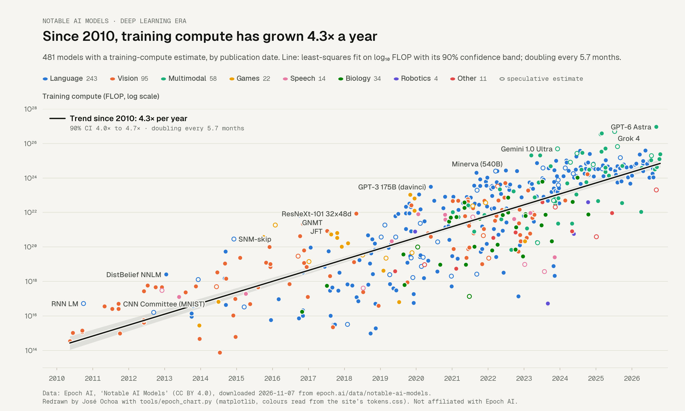
Each behaviour is a rule rather than a per-chart fix, so it would carry to the next explorer.
03 · The stat-card grammar
Epoch’s best interaction is the unit switch on its trend cards. Here it drives three cards computed live from the same JSON as the chart: the number, the sentence and the interval change together.
Before deep learning · 1950–2009
1.5× per year
From 1950 to 2009, training compute of notable models grew 1.5× per year.
Deep learning era · 2010–2026
4.3× per year
Since 2010, training compute of notable models has grown 4.3× per year.
Recent · 2020–2026
5.2× per year
Since 2020, training compute of notable models has grown 5.2× per year.
The 2020+ interval is more than twice as wide as the 2010+ one (0.16 against 0.07 orders of magnitude a year): fewer years, more scatter. The card says that through its interval instead of a caveat paragraph.
Each card is one sentence built from four parts: a lead that names the period, a subject, a verb phrase owned by the unit, and the number. Written down as a template, a researcher can add a card without a designer and every card says the same thing the same way.
| Unit | Number shown | Sentence | 90% interval |
|---|---|---|---|
| Increase/year | 10^b, one decimal, with × | {Lead}, {subject} has grown {n}× per year. | 10^lo× to 10^hi× |
| Doubling time | 12·log₁₀2 / b months, one decimal under 10 | {Lead}, {subject} has doubled every {n} months. | Bounds swap: 12·log₁₀2 / hi to 12·log₁₀2 / lo |
| OOM/year | b, two decimals | {Lead}, {subject} has grown by {n} orders of magnitude a year. | lo to hi |
04 · Same data, in Python
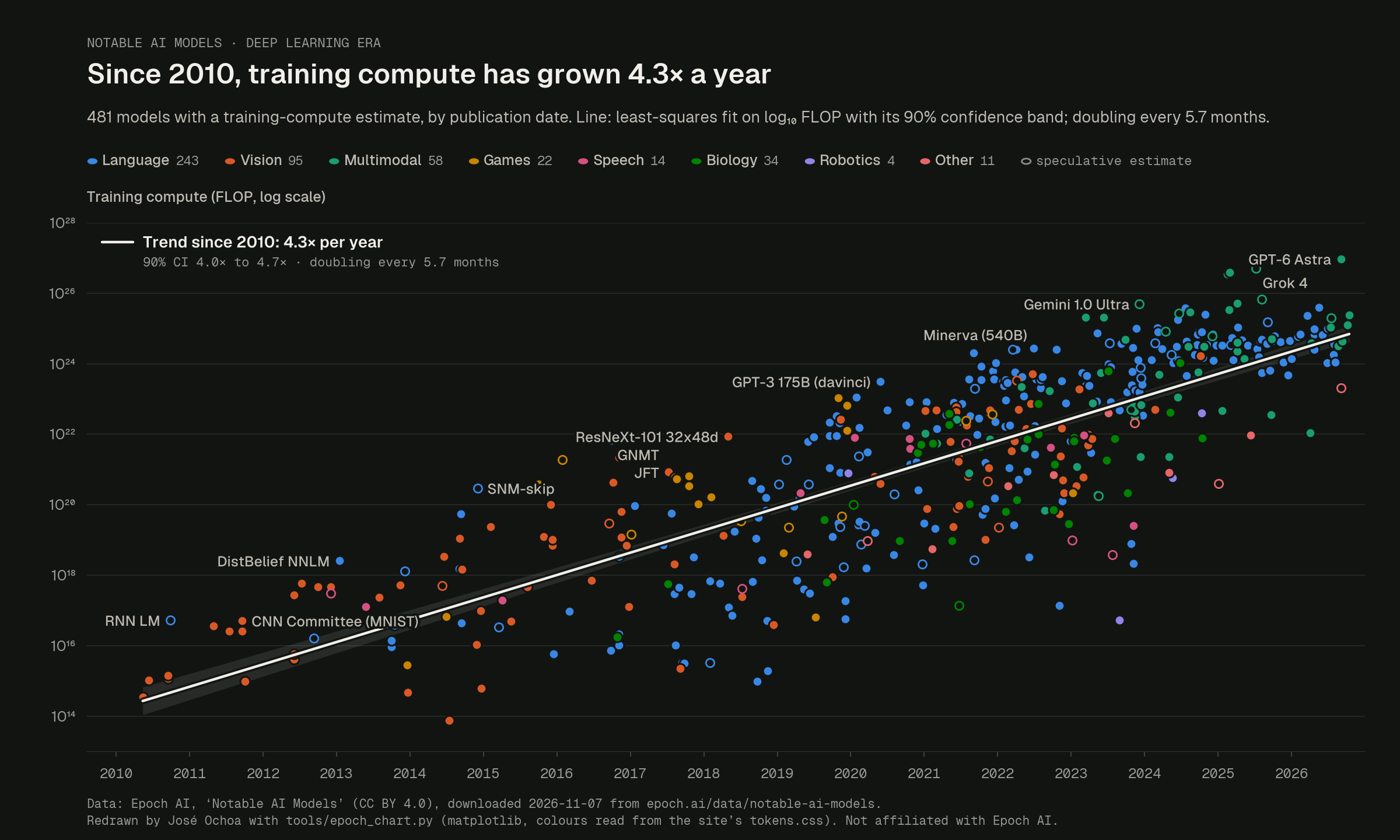
Researchers often need a static figure for a paper, a post or a slide. tools/epoch_chart.py reads the same JSON and this site’s tokens.css, so the PNG has the same colours, fit and label rule as the live chart and cannot drift from it.
"""Matplotlib twin of the Epoch explorer chart.

Renders the same encoding as assets/js/epoch-explorer.js — training compute (log10 FLOP)
against publication date, coloured by domain, OLS trend with a 90% CI band, and the
same label rule — to a static PNG at 2x.

Colours are read from the site's own tokens.css (the light :root block), so the PNG and
the live chart cannot drift apart. Nothing in this file names a hex value.

Usage:
    python tools/epoch_chart.py                       # defaults below, run from site/
    python tools/epoch_chart.py --range all --fonts /path/to/geist-ttf-dir

Requires matplotlib and pandas (pandas only for the CSV-friendly frame).
"""
import argparse
import json
import math
import re
from pathlib import Path

import matplotlib

matplotlib.use("Agg")
import matplotlib.pyplot as plt  # noqa: E402
import pandas as pd  # noqa: E402
from matplotlib import font_manager  # noqa: E402
from matplotlib import patheffects as pe  # noqa: E402

SITE = Path(__file__).resolve().parent.parent
DOMAIN_ORDER = ["Language", "Vision", "Multimodal", "Games", "Speech", "Biology", "Robotics", "Other"]
# key: (axis start with a little padding, first year of data shown, label)
RANGES = {"all": (1948.0, -math.inf, "All time"), "dl": (2009.6, 2010, "Deep learning era"), "recent": (2019.8, 2020, "2020+")}
FIT_FROM = {"all": [(-math.inf, 2010), (2010, math.inf)], "dl": [(2010, math.inf)], "recent": [(2020, math.inf)]}
DATA_END = 2027.0
SUP = str.maketrans("0123456789-", "⁰¹²³⁴⁵⁶⁷⁸⁹⁻")


# ---------------------------------------------------------------- tokens
def read_tokens(css_path, theme="light"):
    css = re.sub(r"/\*.*?\*/", "", Path(css_path).read_text(encoding="utf-8"), flags=re.S)
    toks = {}
    # Light values live in the first top-level rule whose selector list includes a bare `:root`;
    # dark values in the rule for `:root[data-theme="dark"]` (the explicit-toggle scope).
    want = ":root" if theme == "light" else ':root[data-theme="dark"]'
    for sel, body in re.findall(r"([^{}]+)\{([^{}]*)\}", css):
        if want in [s.strip() for s in sel.split(",")] and "--paper:" in body:
            toks = dict(re.findall(r"--([a-z0-9-]+):\s*([^;]+);", body))
            break
    need = ["paper", "paper-2", "ink", "ink-2", "ink-3", "ink-meta", "grid", "axis"] + [f"series-{i}" for i in range(1, 9)]
    missing = [k for k in need if k not in toks]
    if missing:
        raise SystemExit(f"tokens.css is missing {missing}")
    return {k: v.strip() for k, v in toks.items()}


def register_fonts(font_dir):
    if font_dir:
        for f in Path(font_dir).glob("*.ttf"):
            font_manager.fontManager.addfont(str(f))
    names = {f.name for f in font_manager.fontManager.ttflist}
    text = next((n for n in ["Geist", "Inter", "Helvetica Neue", "Arial"] if n in names), "DejaVu Sans")
    mono = next((n for n in ["Geist Mono", "SF Mono", "Menlo", "DejaVu Sans Mono"] if n in names), "DejaVu Sans Mono")
    return text, mono


# ---------------------------------------------------------------- data + stats
def fractional_year(iso):
    ts = pd.Timestamp(iso, tz="UTC")
    return 1970 + ts.value / 1e9 / 86400 / 365.25


def load(path):
    meta_models = json.loads(Path(path).read_text(encoding="utf-8"))
    df = pd.DataFrame(meta_models["models"])
    df["x"] = df["date"].map(fractional_year)
    df["y"] = df["compute"].map(math.log10)
    df["speculative"] = df["confidence"].eq("Speculative")
    return df


def t95(df):
    z = 1.6448536269514722
    return (z + (z**3 + z) / (4 * df) + (5 * z**5 + 16 * z**3 + 3 * z) / (96 * df**2)
            + (3 * z**7 + 19 * z**5 + 17 * z**3 - 15 * z) / (384 * df**3))


def ols(sub):
    n = len(sub)
    mx, my = sub.x.mean(), sub.y.mean()
    sxx = ((sub.x - mx) ** 2).sum()
    b = ((sub.x - mx) * (sub.y - my)).sum() / sxx
    a = my - b * mx
    resid = sub.y - (a + b * sub.x)
    s = math.sqrt((resid**2).sum() / (n - 2))
    se = s / math.sqrt(sxx)
    t = t95(n - 2)
    r2 = 1 - (resid**2).sum() / ((sub.y - my) ** 2).sum()
    return dict(n=n, a=a, b=b, se=se, t=t, lo=b - t * se, hi=b + t * se, r2=r2, mx=mx, sxx=sxx, s=s,
                x0=sub.x.min(), x1=sub.x.max())


def yr_from(key):
    return {"all": 2010, "dl": 2010, "recent": 2020}[key]


def fmt_x(v):
    return f"{v:.0f}" if v >= 10 else f"{v:.1f}"


# ---------------------------------------------------------------- label rule (same as the JS)
def window_ranks(vis):
    xs, cs = vis.x.to_numpy(), vis.compute.to_numpy()
    return {i: int(((abs(xs - xs[k]) <= 0.25) & (cs > cs[k])).sum()) for k, i in enumerate(vis.index)}


def label_order(vis, budget, x0, x1):
    rank = window_ranks(vis)
    pool = vis[[rank[i] <= 2 for i in vis.index]]
    k = max(1, min(budget, 40))
    w = (x1 - x0) / k
    slots = [[] for _ in range(k)]
    for i, row in pool.iterrows():
        slots[min(k - 1, max(0, int((row.x - x0) // w)))].append(i)
    for s in slots:
        s.sort(key=lambda i: (rank[i], -vis.at[i, "compute"]))
    order, rnd = [], 0
    while True:
        batch = [s[rnd] for s in slots if len(s) > rnd]
        if not batch:
            break
        batch.sort(key=lambda i: (rank[i], -vis.at[i, "compute"]))
        order += batch
        rnd += 1
    return order


def truncate(s, n=26):
    if len(s) <= n:
        return s
    cut = s[: n - 1]
    sp = cut.rfind(" ")
    return (cut[:sp] if sp > n * 0.55 else cut).rstrip(" ,(") + "…"


# ---------------------------------------------------------------- draw
def main():
    ap = argparse.ArgumentParser()
    ap.add_argument("--data", default=str(SITE / "data/epoch/notable_models.json"))
    ap.add_argument("--tokens", default=str(SITE / "assets/css/tokens.css"))
    ap.add_argument("--out", default=str(SITE / "assets/img/epoch/notable-models-mpl.png"))
    ap.add_argument("--range", default="dl", choices=sorted(RANGES))
    ap.add_argument("--labels", type=int, default=12)
    ap.add_argument("--fonts", default=None, help="directory of .ttf files to register (e.g. Geist)")
    ap.add_argument("--theme", default="light", choices=["light", "dark"], help="which token block to read")
    args = ap.parse_args()

    T = read_tokens(args.tokens, args.theme)
    SERIES = {d: T[f"series-{i + 1}"] for i, d in enumerate(DOMAIN_ORDER)}
    f_text, f_mono = register_fonts(args.fonts)
    plt.rcParams.update({
        "font.family": [f_text, "DejaVu Sans"], "font.size": 10, "axes.unicode_minus": False,
        "savefig.facecolor": T["paper"], "figure.facecolor": T["paper"],
    })

    df = load(args.data)
    start, data_from, range_label = RANGES[args.range]
    vis = df[df.x >= data_from].copy()
    fits = [dict(ols(vis[(vis.x >= a) & (vis.x < b)]), era="pre" if a == -math.inf else "main")
            for a, b in FIT_FROM[args.range]]

    # Canvas: 1200 x 720 CSS px, saved at dpi 200 -> 2400 x 1440 (2x).
    W, H = 12.0, 7.2
    fig = plt.figure(figsize=(W, H), dpi=100)
    L, R, B, TOP = 0.062, 0.975, 0.105, 0.735
    ax = fig.add_axes([L, B, R - L, TOP - B])
    ax.set_facecolor(T["paper"])
    for sp in ax.spines.values():
        sp.set_visible(False)

    y_lo = math.floor(vis.y.min() - 0.35)
    y_hi = math.ceil(vis.y.max() + 0.25)
    ax.set_xlim(start, DATA_END)
    ax.set_ylim(y_lo, y_hi)

    # grid + axes (powers of ten, one solid hairline per labelled decade)
    plot_h_px = (TOP - B) * H * 100
    step = next((k for k in [1, 2, 3, 4, 5, 6] if plot_h_px / (y_hi - y_lo) * k >= 42), 6)
    yt = list(range(math.ceil(y_lo / step) * step, y_hi + 1, step))
    ax.set_yticks(yt)
    ax.set_yticklabels([f"10{str(e).translate(SUP)}" for e in yt])
    for e in yt:
        ax.axhline(e, color=T["grid"], lw=0.75, zorder=0)
    span = DATA_END - start
    plot_w_px = (R - L) * W * 100
    xs = next((k for k in [1, 2, 5, 10, 20] if plot_w_px / span * k >= 58), 20)
    xt = list(range(int(math.ceil(start / xs) * xs), 2027, xs))
    ax.set_xticks(xt)
    ax.set_xticklabels([str(v) for v in xt])
    ax.axhline(y_lo, color=T["axis"], lw=0.9, zorder=1)
    ax.tick_params(axis="both", length=0, pad=7, labelsize=8.6, labelcolor=T["ink-meta"])
    ax.tick_params(axis="x", length=3, color=T["axis"], width=0.75)
    for lab in ax.get_xticklabels():
        lab.set_fontfamily([f_mono, "DejaVu Sans Mono"])
    for lab in ax.get_yticklabels():
        lab.set_fontsize(9.2)
    ax.text(0, 1.035, "Training compute (FLOP, log scale)", transform=ax.transAxes, ha="left", va="bottom",
            fontsize=9, fontweight=500, color=T["ink-2"])

    if args.range == "all":
        ax.axvspan(2010, DATA_END, color=T["paper-2"], zorder=0, lw=0)
        ax.text(2010.4, y_hi - 0.25, "DEEP LEARNING ERA", fontsize=7.6, family=[f_mono], color=T["ink-meta"], va="top")

    # trend bands under the dots
    for f in fits:
        xx = [f["x0"] + (f["x1"] - f["x0"]) * i / 40 for i in range(41)]
        yy = [f["a"] + f["b"] * v for v in xx]
        hb = [f["t"] * f["s"] * math.sqrt(1 / f["n"] + (v - f["mx"]) ** 2 / f["sxx"]) for v in xx]
        ax.fill_between(xx, [a - h for a, h in zip(yy, hb)], [a + h for a, h in zip(yy, hb)],
                        color=T["ink"] if f["era"] == "main" else T["ink-3"], alpha=0.1, lw=0, zorder=2)

    # dots: solid with a paper ring; speculative estimates hollow
    r_pt = 4.2 * 0.72
    for dom in DOMAIN_ORDER:
        sub = vis[vis.domain_group == dom]
        solid, hollow = sub[~sub.speculative], sub[sub.speculative]
        ax.scatter(solid.x, solid.y, s=(2 * r_pt) ** 2, c=SERIES[dom], edgecolors=T["paper"], linewidths=1.1, zorder=3)
        ax.scatter(hollow.x, hollow.y, s=(2 * r_pt - 0.9) ** 2, facecolors=T["paper"], edgecolors=SERIES[dom], linewidths=1.0, zorder=3)

    # trend lines over the dots, with a paper halo
    halo = [pe.Stroke(linewidth=4.2, foreground=T["paper"], alpha=0.9), pe.Normal()]
    for f in fits:
        ax.plot([f["x0"], f["x1"]], [f["a"] + f["b"] * f["x0"], f["a"] + f["b"] * f["x1"]],
                color=T["ink"] if f["era"] == "main" else T["ink-2"], lw=1.6, solid_capstyle="round", zorder=4, path_effects=halo)

    fig.canvas.draw()
    rend = fig.canvas.get_renderer()
    placed = []  # display-space bboxes

    def free(bb, pad=2):
        if bb.x0 < ax.bbox.x0 + 2 or bb.x1 > ax.bbox.x1 + 18 or bb.y0 < ax.bbox.y0 + 2 or bb.y1 > ax.bbox.y1 - 2:
            return False
        return not any(bb.x0 < p.x1 + pad and bb.x1 + pad > p.x0 and bb.y0 < p.y1 + pad and bb.y1 + pad > p.y0 for p in placed)

    txt_halo = [pe.Stroke(linewidth=3, foreground=T["paper"]), pe.Normal()]

    # trend callout: the upper-left of a rising scatter is empty, so the rate in words and
    # its 90% CI sit there as a keyed legend for the line(s), never on top of the points.
    cy = 0.975
    for f in sorted(fits, key=lambda f: f["era"] != "main"):
        prefix = ("Since 2010: " if f["era"] == "main" else "Before 2010: ") if len(fits) > 1 else f"Trend since {yr_from(args.range)}: "
        rate = f"{prefix}{fmt_x(10 ** f['b'])}× per year"
        ci = f"90% CI {fmt_x(10 ** f['lo'])}× to {fmt_x(10 ** f['hi'])}× · doubling every {12 * math.log10(2) / f['b']:.1f} months"
        ax.plot([0.012, 0.036], [cy - 0.012, cy - 0.012], transform=ax.transAxes, color=T["ink"] if f["era"] == "main" else T["ink-2"],
                lw=1.6, solid_capstyle="round", zorder=6, path_effects=halo)
        t1 = ax.text(0.044, cy, rate, transform=ax.transAxes, fontsize=9.8, fontweight=600, color=T["ink"], va="top", zorder=6, path_effects=txt_halo)
        t2 = ax.text(0.044, cy - 0.04, ci, transform=ax.transAxes, fontsize=7.8, family=[f_mono], color=T["ink-meta"], va="top", zorder=6, path_effects=txt_halo)
        placed.append(matplotlib.transforms.Bbox.union([t1.get_window_extent(rend), t2.get_window_extent(rend)]).expanded(1.04, 1.25))
        cy -= 0.105

    # model labels: same candidate rule as the live chart; greedy, skip on collision
    to_px = ax.transData.transform
    offsets = [(6, -3.5, "left"), (-6, -3.5, "right"), (4, 5, "left"), (-4, 5, "right"), (4, -12, "left"),
               (-4, -12, "right"), (0, 9, "center"), (0, -17, "center")]
    leaders = [(dx, dy, ha) for d in (14, 22, 32) for dx, dy, ha in
               [(d, 0, "left"), (d * .7, d * .7, "left"), (0, d, "center"), (-d * .7, d * .7, "right"),
                (-d, 0, "right"), (-d * .7, -d * .7, "right"), (0, -d - 8, "center"), (d * .7, -d * .7, "left")]]
    count = 0
    for i in label_order(vis, args.labels, start, DATA_END):
        if count >= args.labels:
            break
        row = vis.loc[i]
        name = truncate(row.model)
        done = False
        for k, (dx, dy, ha) in enumerate(offsets + leaders):
            t = ax.annotate(name, (row.x, row.y), xytext=(dx, dy), textcoords="offset points", ha=ha,
                            fontsize=8.8, fontweight=500, color=T["ink-2"], zorder=6, path_effects=txt_halo)
            bb = t.get_window_extent(rend)
            px, py = to_px((row.x, row.y))
            covered = sum(1 for qx, qy in to_px(vis[["x", "y"]].to_numpy())
                          if bb.x0 - 4 < qx < bb.x1 + 4 and bb.y0 - 4 < qy < bb.y1 + 4 and (qx, qy) != (px, py))
            if free(bb) and (covered <= 1 or k >= len(offsets)):
                placed.append(bb)
                if k >= len(offsets):
                    cx = min(max(px, bb.x0), bb.x1)
                    cy = min(max(py, bb.y0), bb.y1)
                    inv = ax.transData.inverted()
                    a = math.atan2(cy - py, cx - px)
                    sx, sy = inv.transform((px + math.cos(a) * 6.5, py + math.sin(a) * 6.5))
                    ex, ey = inv.transform((cx, cy))
                    ax.plot([sx, ex], [sy, ey], color=T["ink-3"], lw=0.75, zorder=5)
                done = True
                break
            t.remove()
        count += done

    # header: eyebrow, title, subtitle, legend
    main_fit = next(f for f in fits if f["era"] == "main")
    yr0 = yr_from(args.range)
    fig.text(L, 0.955, f"NOTABLE AI MODELS · {range_label.upper()}", fontsize=8.2, family=[f_mono], color=T["ink-meta"], va="top")
    fig.text(L, 0.925, f"Since {yr0}, training compute has grown {fmt_x(10 ** main_fit['b'])}× a year",
             fontsize=17, fontweight=600, color=T["ink"], va="top")
    fig.text(L, 0.868, f"{len(vis)} models with a training-compute estimate, by publication date. Line: least-squares fit on log₁₀ FLOP "
             f"with its 90% confidence band; doubling every {12 * math.log10(2) / main_fit['b']:.1f} months.",
             fontsize=9.8, color=T["ink-2"], va="top")
    lx = L
    counts = vis.domain_group.value_counts()
    for dom in DOMAIN_ORDER:
        n = int(counts.get(dom, 0))
        fig.patches.append(matplotlib.patches.Circle((lx + 0.004, 0.808), 0.0036, transform=fig.transFigure,
                                                     facecolor=SERIES[dom], edgecolor="none", figure=fig))
        t = fig.text(lx + 0.011, 0.808, dom, fontsize=9, fontweight=500, color=T["ink-2"], va="center")
        tn = fig.text(t.get_window_extent(rend).x1 / fig.bbox.width + 0.004, 0.808, str(n), fontsize=8,
                      family=[f_mono], color=T["ink-meta"], va="center")
        lx = tn.get_window_extent(rend).x1 / fig.bbox.width + 0.018
    fig.patches.append(matplotlib.patches.Circle((lx + 0.004, 0.808), 0.0032, transform=fig.transFigure,
                                                 facecolor=T["paper"], edgecolor=T["ink-3"], linewidth=1.0, figure=fig))
    fig.text(lx + 0.011, 0.808, "speculative estimate", fontsize=8, family=[f_mono], color=T["ink-meta"], va="center")

    fig.text(L, 0.036, "Data: Epoch AI, ‘Notable AI Models’ (CC BY 4.0), downloaded 2026-11-07 from epoch.ai/data/notable-ai-models.",
             fontsize=7.6, family=[f_mono], color=T["ink-meta"], va="bottom")
    fig.text(L, 0.016, "Redrawn by José Ochoa with tools/epoch_chart.py (matplotlib, colours read from the site’s tokens.css). Not affiliated with Epoch AI.",
             fontsize=7.6, family=[f_mono], color=T["ink-meta"], va="bottom")

    Path(args.out).parent.mkdir(parents=True, exist_ok=True)
    fig.savefig(args.out, dpi=200)
    for f in fits:
        print(f"{f['era']}: n={f['n']} {10 ** f['b']:.3f}x/yr (90% CI {10 ** f['lo']:.3f}-{10 ** f['hi']:.3f}), "
              f"doubling {12 * math.log10(2) / f['b']:.2f} mo, R2={f['r2']:.3f}")
    print("wrote", args.out, "fonts:", f_text, "/", f_mono, "labels:", count)


if __name__ == "__main__":
    main()
To run it: python tools/epoch_chart.py --fonts <geist-dir>. Add --range all for the All time view with both trends.
05 · What I would do next